PaperStation

About

记录自己看到的与计算机视觉，视觉SLAM，机器人，机器学习等相关的论文。如果是比较重要的和自己感兴趣的论文会另开一篇post详细介绍。

2019

Visual SLAM几篇综述

• 基于单目视觉的同时定位与地图构建方法综述

摘 要: 增强现实是一种在现实场景中无缝地融入虚拟物体或信息的技术, 能够比传统的文字、图像和视频等方式更高效、直观地呈现信息，有着非常广泛的应用. 同时定位与地图构建作为增强现实的关键基础技术, 可以用来在未知环境中定位自身方位并同时构建环境三维地图, 从而保证叠加的虚拟物体与现实场景在几何上的一致性. 文中首先简述基于视觉的同时定位与地图构建的基本原理; 然后介绍几个代表性的基于单目视觉的同时定位与地图构建方法并做深入分析和比较; 最后讨论近年来研究热点和发展趋势, 并做总结和展望。

中文综述目前看的比较舒服的一篇，对于visual SLAM有一定了解的人看起来很快，同时也梳理得比较整洁紧凑。

• Visual simultaneous localization and mapping: a survey

Abstract : Visual SLAM (simultaneous localization and mapping) refers to the problem of using images, as the only source of external information, in order to establish the position of a robot, a vehicle, or a moving camera in an environment, and at the same time, construct a representation of the explored zone. SLAM is an essential task for the autonomy of a robot. Nowadays, the problem of SLAM is considered solved when range sensors such as lasers or sonar are used to built 2D maps of small static environments. However SLAM for dynamic, complex and large scale environments, using vision as the sole external sensor, is an active area of research. The computer vision techniques employed in visual SLAM, such as detection, description and matching of salient features, image recognition and retrieval, among others, are still susceptible of improvement. The objective of this article is to provide new researchers in the field of visual SLAM a brief and comprehensible review of the state-of-the-art.

这是一篇非常棒的综述，对于入门的人非常友好，几乎没有数学公式，只是对slam中的各个问题和模块进行了分解，词汇也不复杂，读起来很快。但是缺点是不是很新，而且深度不够。

• Past, Present, and Future of Simultaneous Localization And Mapping: Towards the Robust-Perception Age

Abstract—Simultaneous Localization and Mapping (SLAM) consists in the concurrent construction of a model of the environment (the map), and the estimation of the state of the robot moving within it. The SLAM community has made astonishing progress over the last 30 years, enabling large-scale real-world applications, and witnessing a steady transition of this technology to industry. We survey the current state of SLAM. We start by presenting what is now the de-facto standard formulation for SLAM. We then review related work, covering a broad set of topics including robustness and scalability in long-term mapping, metric and semantic representations for mapping, theoretical performance guarantees, active SLAM and exploration, and other new frontiers. This paper simultaneously serves as a position paper and tutorial to those who are users of SLAM. By looking at the published research with a critical eye, we delineate open challenges and new research issues, that still deserve careful scientific investigation. The paper also contains the authors’ take on two questions that often animate discussions during robotics conferences: Do robots need SLAM? and Is SLAM solved?

这个综述相对难说难度点，但是写的非常好，毕竟作者都是有名的大佬。比较难得的是，这篇综述不仅梳理了slam的发展历程和技术现状，还提出了一些"open problem"，表明了自己的的观点，详细地阐述了视觉SLAM现在的挑战以及未来可能的应对办法，虽然有些问题是显而易见的。此外，该综述中也提供了很多参考文献，尤其是对于场景识别中的感知混叠以及滤波器优化和非线性优化的比较，以及因子图的功效，后续都值得研究一下。

• FutureMapping: The Computational Structure of Spatial AI Systems,Andrew J. Davison

We discuss and predict the evolution of Simultaneous Localisation and Mapping (SLAM) into a general geometric and semantic ‘Spatial AI’ perception capability for intelligent embodied devices. A big gap remains between the visual perception performance that devices such as augmented reality eyewear or consumer robots will require and what is possible within the constraints imposed by real products. Co-design of algorithms, processors and sensors will be needed. We explore the computational structure of current and future Spatial AI algorithms and consider this within the landscape of ongoing hardware developments.

blog

• FutureMapping 2: Gaussian Belief Propagation for Spatial AI

blog

• Ongoing Evolution of Visual SLAM from Geometry to Deep Learning: Challenges and Opportunities

这篇综述主要关注的是深度学习在slam中的应用，先介绍了几种常见的模型，即CNN, RNN和encoder, decoder，然后列举了一些slam常用的dataset，包括KITTI, TUM, NYU等，接着分块介绍深度学习在depth estimation, pose estimation, ego-motion estimation, relocalization, sensor fusion, semantic mapping方面的应用概况，总的来说在位姿估计，深度尺度估计，回环检测重定位，地图构建这几个方面着手，论文最后提出了一些存在的挑战和思路，总体来说介绍的还是挺全的，列举的文章也很经典。但是总觉得深度不够，像是一种在知乎上回答问题的方式。虽然值得看，不过等到以后发现了更好的综述再来替换吧。

• A Survey of Simultaneous Localization and Mapping

Focal Loss

• paper
• code

loss的具体形式为：$criterion= \alpha(1-a)^{\gamma}y \ln a + (1-\alpha)a^{\gamma}(1-y) \ln (1-a)$，主要的作用就是提高对假阴性的惩罚力度，在论文中作者指出，对于设计的RetinaNet，超参数$\alpha=2, \gamma=0.25$效果最好（分类目标检测阶段的前景和背景分离），在我实际的二分类使用中，效果并不是十分突出，参数的调节是个技术活，否则很容易使得假阳性很高，不过这可能也是和数据集有关。

pytorch代码如下：

import torch
from torch import nn
#自定义的模型和loss都要继承nn.Module类
class BFocalLoss(nn.Module):
      def __init__(self, gamma=2, alpha=0.25):
          super(BFocalLoss, self).__init__()
          self.gamma = gamma
          self.alpha = alpha
      def forward(self, inputs, targets):
          pt = nn.Softmax(input, dim=1)
          p = pt[:,1]
          loss = -self.alpha * (1-p) ** self.gamma*(target*torch.log(p+1e-12)) - \
                 (1-self.alpha)*p**self.gamma*((1-target)*torch.log(1-p+1e-12))
          return loss.mean()
      

medium上一篇blog对flocal loss进行了阐释。

Deep Learning in Tumor Metastatic on Medicine Image

两篇深度学习在乳腺癌细胞转移检测的论文：

• Deep Learning for Identifying Metastatic Breast Cancer
• Detecting Cancer Metastases on Gigapixel Pathology Images

医学图像处理与自然图像处理不同，一般来说由于设备的原因，可能病灶特征不是特别容易区分，也不是很明显，因此ImageNet上的预训练模型可能不是很有用。医学图像方面由于图像数量少，标注成本高，所以用的tricks比较多，要根据具体的要求和数据采集情况分析，比如痰涂片载玻片图像，一般得到的数据集可能是组与组之间是连续的特征，就像视频中连续帧的图像，差别不会很大，因此标注的时候可能只需要根据采集的组进行少量标注就可以，进行弱监督训练，也可能达到很不错的分类精度。

• 特定的数据增强，RGB-HSV转换，color normalization
• slide选取patches放大不同尺度，多尺度输入
• 原始样本旋转90，180，270度，left-right flip之后再旋转90，180，270度，这样就扩增到了8倍大小。然后进行图像色调的调整，包括对比度，亮度，饱和度等。
• FROC 而不是ROC和AUC（performance衡量标准）
• 减少计算，移除背景patches
• 随机森林提取heatmap特征

Mixup

• paper
• code

adversarial examples， ERM（经验风险最小化）准则不能很好的适用，数据增强，VRM（近邻风险最小化），插值生成对抗样本和标签

$\widetilde x = \lambda x_{i} + (1-\lambda)x_{j}\\ \widetilde y = \lambda y_{i} + (1-\lambda)y_{j} \\$

对交叉熵损失函数和Focal Loss而言，可以直接取出$y_{i}, y_{j}$对其损失函数进行插值(数学上可以推导)

$loss = \lambda \cdot criterion(\widetilde x, y_{i}) + (1-\lambda) \cdot criterion(\widetilde x, y_{j})$

The mixup vicinal distribution can be understood as a form of data augmentation that encourages the model f to behave linearly in-between training examples. We argue that this linear behaviour reduces the amount of undesirable oscillations when predicting outside the training examples. Also, linearity is a good inductive bias from the perspective of Occam’s razor, since it is one of the simplest possible behaviors.

论文指出，mixup可以控制模型复杂度，也就是说模型在ERM情况下不断训练会记住training data，导致泛化能力差，而mixup通过随机pairing插值融合，生成对抗样本可以有效的缓解这种情况。而且通过大量的实验，证明mixup确实有效果，而且在各个领域都还不错，此外可以和dropout等控制模型复杂度方法相结合。

We have shown that mixup is a form of vicinal risk minimization, which trains on virtual examples
constructed as the linear interpolation of two random examples from the training set and their labels. Incorporating mixup into existing training pipelines reduces to a few lines of code, and introduces little or no computational overhead. Throughout an extensive evaluation, we have shown that mixup improves the generalization error of state-of-the-art models on ImageNet, CIFAR, speech, and tabular datasets. Furthermore, mixup helps to combat memorization of corrupt labels, sensitivity to adversarial examples, and instability in adversarial training.

在图像上的训练trick: 训练时每个epoch都采用mixup，$\lambda$的取值由$Beta(\alpha,\alpha)$函数随机指定，$\alpha$是hyper-parameter，论文中指出在imagNet上的值在[0.1, 0.4]之间，在CIFAR上取的是1，此外，网络结构加深和训练周期的加长都会使得最终的泛化效果比较好。但是论文中没有将为什么选用$beta$函数去生成$\lambda$，优化器选的是带动量的SGD，其中learning rate会随着指定的epoch范围进行下降，且没有使用drop out。

numpy.random.beta()是对beta分布进行随机采样，下式是beta分布的概率密度函数，当$\alpha$的取值越大时，取样的值基本就会往0.5靠近，这时候似乎就退化成sample pairing。

$\lambda = f(x ; a, b)=\frac{1}{B(\alpha, \beta)} x^{\alpha-1}(1-x)^{\beta-1} \\ B(\alpha, \beta)=\int_{0}^{1} t^{\alpha-1}(1-t)^{\beta-1} dt$

mixup与IBM的一篇文章sample pairing的想法很类似，而且提出的时间都差不多，不过sample pairing是随机将两幅图片平均插值，但是label不变，等于是引入噪声，而且训练的trick也比较多，可以参考这篇博客的实验。

如果加入warmup，学习率随指定epoch下降，weight decay=$10^{-4}$（对于mixup，小的weight decay效果 更好)，此外超参$\alpha$的取值越大，训练集的loss会越大，但是泛化能力就会越好。但是具体的数据集可能training loss变化趋势不同，可能随着$\alpha$的增加急剧增加，也可能不怎么变化，因此最佳的位置，作者也提出了疑问，放在了discussion中，他们猜测可能大容量模型可能会对大取值$\alpha$的适应度好点。

In our experiments, the following trend is consistent: with increasingly large $\alpha$, the training error on
real data increases, while the generalization gap decreases.

---

2020.3，另有两篇images mixture的文章，分别是关于有监督和无监督领域的：

SuperMix: Supervising the Mixing Data Augmentation

Rethinking Image Mixture for Unsupervised Visual Representation Learning

Thoracic Disease Identification and Localization with Limited Supervision

paper

code

这是平安科技和李飞飞合作的论文，主要是通过图片级label标注和少量框标注来达到病灶regions显示的目的，生成heatmap和类别判定。

Given images with disease labels and limited bounding box information, we aim to design a unified model that simultaneously produces disease identification and localization.

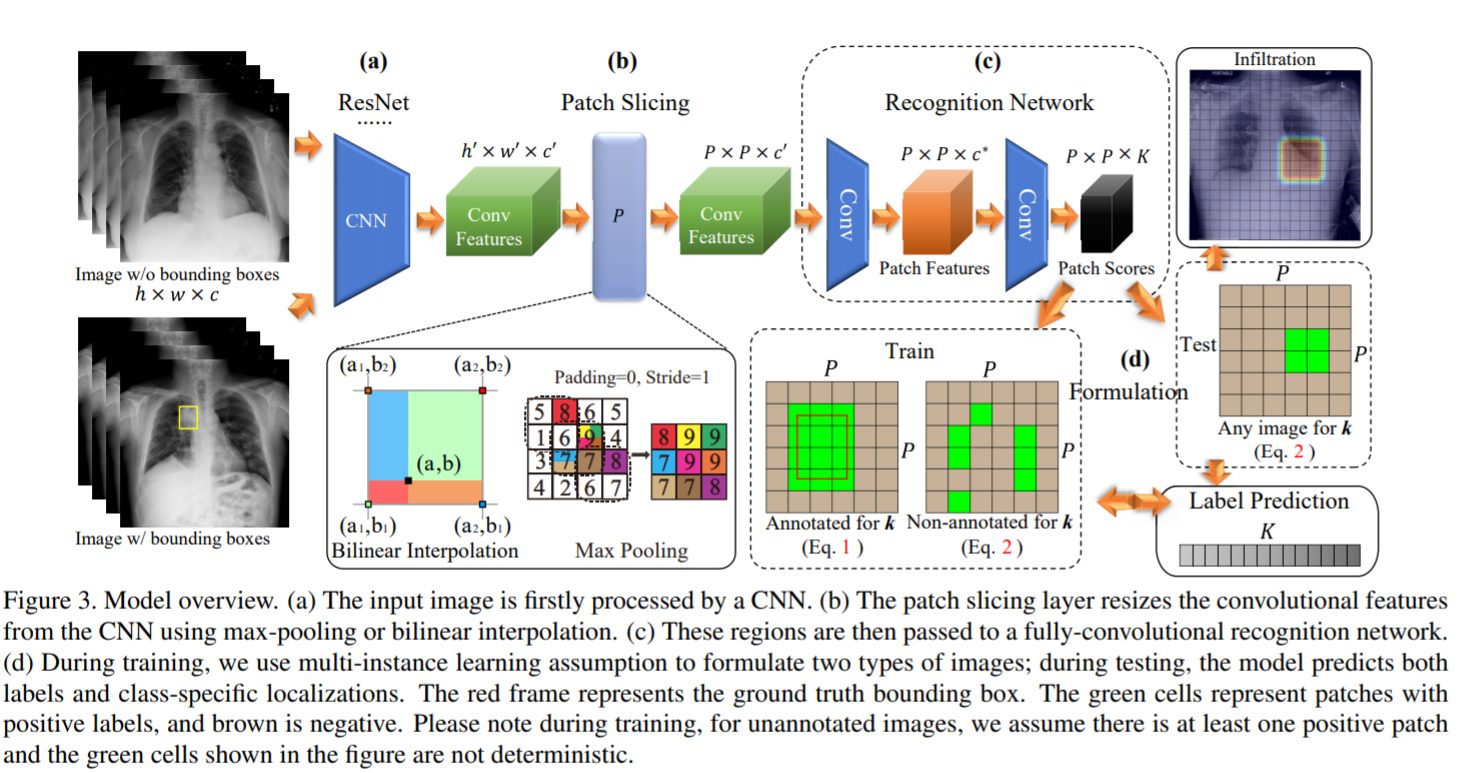
大致的网络结构是利用resnet backbone进行下采样，生成$P \times P$的feature map，然后对应原图的空间尺寸，有框的话就进行像素级的比对预测，没框但是有图片级的label的话那么这张图片中肯定存在至少一个patch对应于这种疾病，就直接根据概率进行预测。（多实例学习）

• 利用resnet结构，去掉global pooling和fc层，利用卷积block下采样图片，得到feature map
• 不同size的input图片最后得到的feature map尺寸不同，为了得到设定的patch大小，大的feature map进行maxpooling进行下采样，小的利用bilinear interpolation（双线性插值）扩大
• feature map送入全卷积网络，先通过$3 \times 3$的卷积层，卷积核大小$c^{*}=512$，然后在送入$1 \times 1$的卷积层，生成$P \times P \times K$的feature map，也就是$K$个类别的预测图，根据每个图上预测的概率值进行判断属于哪个类别。（output map与target map进行loss定位回归）

损失函数就是利用权重$\lambda$调节框监督和无框标注的重要程度，利用二元参数$\eta$来选择图片的监督信息对应的loss函数。

对于每个patch在之前的过程中都预测出了对应的score，在定位阶段设置一个阈值，只要score大于该值即可认为它是positive patch，论文中的阈值设置为0.5。之前论文中提到，并不预测出严格的位置来，而是一个大概区域。因为经过阈值判定的结果并不会精确地分布在一个规则的矩形框之中。

个人觉得这篇文章的两个亮点在于：

• 医疗影像处理，论文实验做的也不少
• 不同的监督信息混合，多实例学习，得到区域分割和类别判断的效果

但是通篇读下来觉得收获并不是很大，废话比较多，让人耳目一新的东西并不多，如果不是Feifei Li挂名的话，可能登不上CVPR。不过实习的项目想拿这篇文章的思想来做些东西，于是便选择读了。

FCN: Fully Convolutional Networks for Semantic Segmentation

paper

code

开始之前先了解下上采样中的反卷积(deconvoltion)方法（一般有双线性插值，反卷积和反池化三种方法）。

实际上，转置卷积(transposed convolution)这种叫法可能更为合适。因为反卷积的数学含义，通过反卷积可以将通过卷积的输出信号，完全还原输入信号，而事实是，转置卷积只能还原shape大小，不能还原value. 知乎专栏, 知乎

转置卷积是一种特殊的正向卷积，先按照一定的比例通过补0来扩大输入图像的尺寸，接着旋转卷积核，再进行正向卷积。

输入元素矩阵$X$，输出元素矩阵$Y$，正向卷积的矩阵为$C$，则正常的卷积操作过程为：$Y = CX$，反卷积的操作就是要对这个矩阵运算过程进行逆运算，即: $X=C^{T}Y$。但是此操作只会恢复矩阵大小，并不会恢复元素值。

转置卷积的公式：

\begin{align} & o = \text{size of output} \\ &i = \text{size of input} \\ &p = \text{padding} \\ &s = \text{strides} \end{align}

对于正常卷积：$o=[(i+2p-k)/s]+1$

对于转置卷积：

如果$(o+2p-k) \% s =0$，则可以通过$0 = s(i-1)-2p+k $来确定卷积核参数，

如果$(o+2p-k) \% s \not =0$，则可以通过$o = s(i-1)-2p+k+(0+2p-k)% s $来确定卷积核参数

FCN是深度学习+语义分割领域的的milestone论文。语义分割的基本思想和分类相同，只不过是预测图像中的每个像素的所属类别（对类别进行数字编码，加上无关背景，总共是$n_{classes}+1$类，然后每个类别可以用不同的颜色显示），然后计算像素级别的loss，再进行back propagation。FCN也是这种训练方式，最后生成的特征图的个数是类别个数，所有特征图的每个像素进行log_softmax预测属于哪种类别，最后解码成设定的RGB图像。

architecture+implementation:

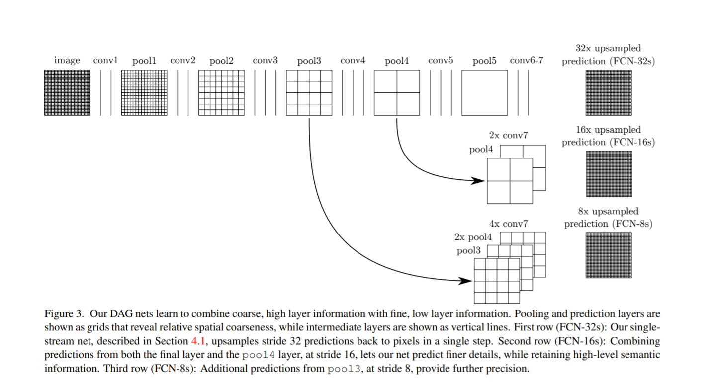
原文对backbone的选择，以及训练集选择，数据预处理，训练数据采样，训练过程中的超参等进行了实验，因此实验内容还是十分丰富的，最终表现好的backbone 是VGG-16，然后实验之后认为利用卷积层提取特征，pooling层下采样5次后预测的精度比较高，结构中亮点在于skip connections，采样较少的feature map尺寸大，保留了比较多的local信息，对小物体表式比较好，采样较多的feature map尺寸小，特征层级高，体现的是global信息，然而对小物体表示比较差，因此lower layer和higher layer融合可以比较好的全面表示图像的语义信息，这个结构提出了这个思考，同时也进行了实验，分别给出不融合，融合一层，融合两层的结构，看各自的表现如何。实验也表明FCN-8s的精度最好，而且越融合精度提升的点不大，但是会使得最后的结果更加smooth。

训练过程中权重初始化是个很重要的trick，论文是先利用在ImageNet上预训练过的模型去掉最后的全连接层来初始化权重，然后进行后面三个pooling过的feature map对应融合再去最后的上采样（full卷积，即反卷积）得到$c\times h \times w$的图像。FCN中的full卷积方式是先对特征图进行padding，用0填充，然后再进行正常的卷积操作，得到上采样的结果，反卷积层的权重初始化也是个很重要的部份，论文中说使用随机初始化效果不怎么样，这里可以使用bilinear kernel，此函数在pytorch中也有，下面的代码讲解中也有具体介绍。对于最后的loss计算，图像的每个像素点有21（针对pascal VOC数据集，最后网络输出的是$c\times h \times w$个特征图，$c=21$）个归一化概率值，最大的索引代表类别数字，也就是说是每个像素会进行一个loss计算，每个图像有$h\times w$个像素值，最会全部加起来进行backpropagation，等于是图片级分类问题中的一个"batch"操作。

pytorch实现FCN代码讲解

blog详解FCN网络

metric：

假设$n_{ij}$是将类别$i$的像素预测成类别$j$的像素的个数，$n_{cl}$是物体的类别数，$t_{i}=\sum _{j}n_{ij}$是预测成像素$i$的总个数（包含正确预测的和把其他类别预测成$i$的）

• pixel accuracy: $\sum_{i} n_{i i} / \sum_{i} t_{i}$

• mean accuracy: $\left(1 / n_{\mathrm{cl}}\right) \sum_{i} n_{i i} / t_{i}$

• mean IU(region intersection over union): $\left(1 / n_{\mathrm{cl}}\right) \sum_{i} n_{i i} /\left(t_{i}+\sum_{j} n_{j i}-n_{i i}\right)$

• frequency weighted IU: $\left(\sum_{k} t_{k}\right)^{-1} \sum_{i} t_{i} n_{i i} /\left(t_{i}+\sum_{j} n_{j i}-n_{i i}\right)$

FCN在语义分割（semantic segmentation）和场景理解（scene parsing）领域中是一项非常重要的工作，模型思想很简单，同时也是非常具有逻辑性的，但是论文读起来个人感觉不是特别顺畅，可能是自己的原因，觉得讲得比较乱，可能是因为作者做了很多的实验性尝试去试着提高精度，但是都没什么太大的用处，但是又不得不写出来突出工作量的缘故。抛开论文不谈，FCN的意义是重大的，毕竟是从0到1的工作，而且在代码上也有不少工作，尤其是相对图像级别的分类任务而言，有很多流程和细节部份需要注意，否则训练可能会得不到好的效果，比如数据读取数据预处理部份（图像级label-RGB值编码-类别数字编码对应抽取对应，为了进行batch训练对图像和label对应crop等），以及权重初始化，卷积核设计等，自己完整写一遍FCN的代码并且调试出好的结果肯定会大有裨益。

BoxSup: Exploiting Bounding Boxes to Supervise Convolutional Networks for Semantic Segmentation

paper

这篇文章的思路和后面的deepcut处理医学图像分割的思路很像（boundingbox supervised），此外伯克利大学Jitendra Malik等人2014的一篇论文SDS也跟此论文的结构很类似，也使用MCG进行预选mask提取。

作者利用bounding box进行弱监督学习semantic segmentation，最后的结果令人满意，如果进行半监督（1/10的数据使用像素级标注，9/10的数据使用bounding box进行标注）训练，最后的结果甚至可以达到STOA的水平（2015年）。作者认为效果好的原因在于bounding box监督的方式使得网络提高了物体识别的准确率，这样的话就会容易将foreground和background分开，网络也会将特征学习集中在instance上面，得到的特征质量也会比较高。

模型的大致框架是：先利用region proposal(MCG, Multiscale Combinatorial Grouping)得到candidate segmentation mask，然后利用FCN训练得到coarse的分割结果，过CRF进行轮廓平滑，然后再利用这个estimation作为新的label丢进网络进行训练，iterative training得到最后的分割结果。

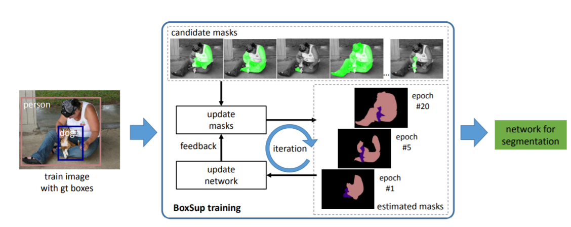
模型实现的重点在于一是利用MCG等region proposal方法生成候选mask，然后进行随机sampling，分割训练backbone用的是FCN，之后经过CRF（不是denseCRF）后处理，一个epoch遍历完所有图片后，预测生成的mask重新作为原图的label，迭代进行训练。等于是两个网络进行end-to-end训练学习

loss function:

$\min _{\theta,\left\{l_{S}\right\}} \sum\left(\mathcal{E}_{o}+\lambda \mathcal{E}_{r}\right)$

$\mathcal{E}_{o}=\frac{1}{N} \sum_{S}(1-\operatorname{IoU}(B, S)) \delta\left(l_{B}, l_{S}\right)$

$\mathcal{E}_{r}=\sum_{p} e\left(X_{\theta}(p), l_{S}(p)\right)$

第一个loss$\mathcal{E}_{0}$是region proposal部份生成的候选mask的惩罚函数，采用的是交并比IoU，取值在[0,1]之间，$l_{B}, l_{S}$

分别代表bounding box和semantic mask的标签，因为可能有多个类别，只计算每个类别的bounding box和semantic mask代表同样类别的交并比，因此，如果是同类$\delta$就是1，否则是0，$1/N$是为了归一化（或者正则化，whatever）。

第二个loss是标准的semantic segmentation中的像素级loss，每个像素进行类别上的cross-entropy，其中$X_{\theta}(p)$代表FCN网络预测的标签，$l_{s}(p)$代表用来全监督的label，第一次是MCG生成的候选mask，后面则是网络预测并进行CRF后处理后覆盖的mask。

最后将两个网络的loss加在一起，并设置权重系数$\lambda$来调节两者对整体模型的贡献度，按直觉说，应该是FCN等backbone预测pixel标签部分更为重要，因此$\lambda$应当大于1，论文中此超参给的值是3。

模型的核心点除了迭代标签之外，就是候选mask的生成以及分配相应的label给candidate segments，这些问题需要弄清楚：

The candidate segments are used to update the deep convolutional network. The semantic features learned by the network are then used to pick better candidates. This procedure is iterated.

As a pre-processing, we use a region proposal method to generate segmentation masks. We adopt Multiscale Combinatorial Grouping (MCG) by default, while other methods are also evaluated. For all experiments we use 2k candidates on average per image as a common practice. The proposal candidate masks are fixed throughout the training procedure. But during training, each candidate
mask will be assigned a label which can be a semantic category or background. The labels assigned to the masks will be updated.

分配标签问题文中是利用贪心迭代算法（greedy iterative solution）来寻找局部最优值：

With the network parameters $\theta$ fixed, we update the semantic labeling $\left\{l_{s}\right\}$for all candidate segments. As mentioned above, we only consider the case in which one ground-truth bounding box can “activate” (i.e., assign anon-background label to) one and only one candidate. As such, we can simply update the semantic labeling by selecting a single candidate segment for each ground-truth bounding box, such that its cost $\mathcal{E_{0}}+\lambda \mathcal{E_{r}}$is the smallest among all candidates. The selected segment is assigned the groundtruth semantic label associated with that bounding box. All other pixels are assigned the background label.

The above winner-takes-all selection tends to repeatedly use the same or very similar candidate segments, and the optimization procedure may be trapped in poor local optima. To increase the sample variance for better stochastic training, we further adopt a random sampling method to select the candidate segment for each ground-truth bounding box. Instead of selecting the single segment with the smallest cost $\mathcal{E_{0}}+\lambda \mathcal{E_{r}}$, we randomly sample a segment from the first $k$ segments with the smallest costs. In this paper we use $k = 5$. This random sampling strategy improves the accuracy by about 2% on the validation set.

然而我还没研究到MCG，此论文也没有开源代码，我只能粗略理解为先是通过MCG为每张图片生成2K的candidate segment region proposal，然后对像素标签，训练完并进行了CRF 后处理的时候根据损失函数去找比较小的几个candidate，随机抽取K个进行重新assign标签，然后再迭代训练。这里有两个疑问待解决：一个是生成的2k个proposal应该是在每个类别上都有重复的，这样的话怎么一个bounding box对应一个segment进行监督学习；第二个是原来的update 方法是利用损失函数最小的那个框对去更新segment，，然后再训练，这个很直观，可以理解，但是论文中说为了防止"winner takes all"的误区，也就是陷入局部最优值，随机抽取了k个最小的segments，然后进行迭代，这样的话就又等于是拿出了多个candidate去监督吗？目前我还没弄明白具体的实现细节。。

增加带bounding box标注的数据显著提高了模型的performance：

recognition error that is due to confusions of recognizing object categories;

boundary error that is due to misalignments of pixel-level labels on object boundaries

主要原因还是增大了数据量使得模型对特征提取更加健壮，能够更好地进行object recognition

Simple Does It: Weakly Supervised Instance and Semantic Segmentation

paper

github1

github2

这篇文章在BoxSup之后，细节部份写得要比前者详细的多，虽然方法相似，但是很值得一读，可以得到不少收获。

直接box或者其他region proposal生成segments，DeepMask作为instance segmentation参考模型，重构semantic segmentation model DeepLabv2去进行instance segmentation，训练部分常规操作，最后还对集中segment生成方法进行了比较。

From boxes to semantic labels:

C1 Background 未被框包围的像素认为是background

C2 Object extend 框包围了整个object，但是物体的形状可以作为另外一个先验信息，比如椭圆形状的病菌就会看起来更像一个细长的bar，模型会将这个size信息用在模型学习中

C3 Objectness 除了框带来的区域和范围信息，还有两个典型的先验，即空间连续信息和相较于background对比明显的物体轮廓信息。通常情况下可以通过segment proposal(GrabCut，MCG等)来枚举并排序一些比较像的大部分处于框内的物体形状。

methods:

naive的转换标签是将box里面的全部像素assign为对应类别，外面的为背景，如果两个框交叉了，那么重合的部分是交叉框的标签（也可以从图片上直观看出），之后进行recursive training，预测的结果去update label，论文中给的结果看起来比想象中要好不少，主要原因是training被去噪和标注以及先验信息进行加强了，主要是对模型预测的结果采用了三个后处理方法：预测部份pixel在bounding box之外的全部置为background；预测部份和bounding box计算IoU，如果小于50%，重新把整个box变成像素标签（等于是回到一开始的label）；预测部份过DenseCRF平滑轮廓（use DenseCRF with the DeepLabv1 parameters），这是很重要的一步，对提升performance很有帮助。以上方法作为论文的两个baseline，名叫Naive（不带post-processing)和Box

另外一个利用矩形标注的方法是$Box^{i}$，引入了ignore regions，也就是将bounding box内20%的区域进行pixel标注，其他区域作为忽视区域，这样的话可能会减少原始输入标签的噪声，同时这20%的标签也会尽可能overlap对应的object，后续也会经过上文中的三个post-processing阶段。

GrabCut+方法是参考Grabcut这个region proposal 技巧去生成较bounding box更为精细的分割，论文是用了HED边缘检测方法（ICCV2015，paper, code）而不是典型的RGB颜色差异去分割预选segments，因此论文称为GrabCut+方法，同时也仿照了$Box^{i}$方法提出了另一个baseline$GrabCut^{i}$（区域的比例阈值设定所有不同）。此外，也采取了另一种当时比较流行的region proposal方法MCG，这也是BoxSup中采用的方法，一个baseline是单用MCG方法，另一个是和**GrabCut+**结合，即$MCG \cap GrabCut+$，等于是简单的ensemble投票方法。

语义分割方面使用的是Deeplab模型，实例分割用的是DeepMask模型，论文也对这些模型实现方法进行了修改，以适合本情况。论文在单数据集，多数据集，以及前处理生成segments上做了很多对比实验，总体来说操作上要比BoxSup简单些，而且效果也很有竞争力。

FutureMapping

SLAM领域大佬Andrew Davison的新作

FutureMapping

FutureMapping2

目标检测R-CNN系列

R-CNN—>SPPNet–>Fast R-CNN–>Faster R-CNN–>OHEM

R-FCN, FPN

2020

Deep GrabCut for Object Selection

paper

code

image+Euclidean distance map

Holistically-Nested Edge Detection

paper

code: tf, caffe, pytorch

Seed, Expand and Constrain: Three Principles for Weakly-Supervised Image Segmentation

paper

Weakly-Supervised Semantic Segmentation by Iteratively Mining Common Object Features

paper

U-Net: Convolutional Networks for Biomedical Image Segmentation

paper

code1

code2

U-Net family

U-Net是医学图像分割领域效果很好的一个网络架构，对称的下采样和上采样操作以及skip connections保证了特征图既包含了低层级的特征，也包含了高层级的语义特征，适合单一和图像梯度复杂的医学图像，实际在自然图像中表现也不错。（知乎：为什么U-Net在医学图像分割领域表现不错）

U-Net++: A Nested U-Net Architecture for Medical Image Segmentation

paper

code

blog

CAM–Learning Deep Features for Discriminative Localization

• paper
• [code]

卷积单元即使在没有监督下也可以detect object，但是这种能力会在后面的全连接层下消失，通过global average pooling可以保持这种能力。

class activation mapping

CRFasRNN

[paper]

Efficient Inference in Fully Connected CRFs with Gaussian Edge Potentials

paper

code

$E(x)=\sum_{i} \psi_{u}\left(x_{i}\right)+\sum_{i<j} \psi_{p}\left(x_{i}, x_{j}\right)$

$\psi_{p}\left(x_{i}, x_{j}\right)=\mu\left(x_{i}, x_{j}\right) \sum_{m=1}^{K} w^{(m)} k^{(m)}\left(f_{i}, f_{j}\right)$

$k^{(m)}\left(f_{i}, f_{j}\right)=w^{(1)} \exp \left(-\frac{\left|p_{i}-p_{j}\right|^{2}}{2 \theta_{\alpha}^{2}}-\frac{\left|I_{i}-I_{j}\right|^{2}}{2 \theta_{\beta}^{2}}\right)+w^{(2)} \exp \left(-\frac{\left|p_{i}-p_{j}\right|^{2}}{2 \theta_{\gamma}^{2}}\right)$

Multiscale Combinatorial Grouping for Image Segmentation and

Object Proposal Generation
paper

code

Weakly- and Semi-Supervised Learning of a Deep Convolutional Network for Semantic Image Segmentation

paper

Learning to Reweight Examples for Robust Deep Learning

paper

code

batch-reweight

Detecting Lesion Bounding Ellipses With Gaussian Proposal Networks(GPN)

椭圆标注的目标检测，比如医学图像中deep-lesion，人脸检测。

一种直觉的方法是通过三个点（中心点，长轴点，短轴点）和一个旋转角度$\tan\theta$，仿照faster r-cnn来进行回归，但是长短轴比例ration较大或者接近与1的时候，就会要求角度预测的很准确或者不需要准确，而且two-stage效率比较低。

GPN源于二维高斯分布，通过ground truth的概率分布图的等高线（椭圆）来和预测的做距离上的regression，这样就大大降低了参数量，对于旋转的情况，利用rotation matrix来进行坐标系的平移（关键词：协方差矩阵，KLD损失函数，概率密度函数，像素密度<foreground,backgroud>)

Class-Balanced Loss Based on Effective Number of Samples

paper

code

Tell Me Where to Look: Guided Attention Inference Network

paper

code

Dice Loss

Deep Learning + Visual Odometry

• [deepvo]

• [code]

• [sfmlearner]

• [code]

• [undeepvo]

• [code]

• GANvo

• [code]

• [SGANvo](